Category: FTN

  • Faster-Than-Nyquist Signaling: Systems Model and Project Goals

    Back to project page

    Back to welcome page

    Introduction

    Previously, I gave a primer on Faster-Than-Nyquist (FTN) systems and how they improve on the current state of the art. In this blog, we will discuss the high level of the FTN system model as well as the goals my friend and I have for the FTN project.

    A side note for this and future articles: These articles build off each other. Please refer to previous blogs to help in understanding these terms if you are confused. I do my best to explain the jargon as simply as I can in those articles, but if you still need clarification, you are more than welcome to send an email to dscmece@gmail.com. I will do my best to respond in a timely manner.

    FTN System Model

    As stated in the previous blog, FTN signaling involves us sending a pulse every TFTN = τ/2W seconds. A simpler way for us to say this (and the way I will say it from now on), is that we are looking to transmit every τT seconds instead of every T seconds, where 0 < τ< 1. Since this signaling scheme sacrifices orthogonality, we need some way to mathematically represent the interference between our data symbols (called intersymbol interference – ISI). To do this, we will look at the communication systems model in Figure 1 for reference.

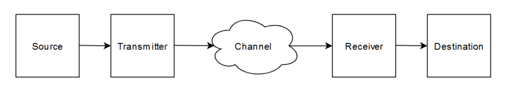
    The main parts of interest for us here are the transmitter, channel, and receiver. For simplicity, let’s stick with a standard Nyquist rate system. Starting with the transmitter, we know it is going to send some data sequence. Mathematically, we write it as a column vector containing the data symbols. We will call this vector \( \bar{x}\).

    When we deal with our transmitted data, we treat it as noiseless and shift the non-ideal aspects of the transmitter design (e.g. temperature induced noise in an IC) to the channel. The most common model we use for the channel is the Additive White Gaussian Noise (AWGN) model. For the uninitiated, AWGN is noise which is distributed according to a Gaussian distribution (AKA Normal distribution or the “Bell Curve” distribution) which is added onto the transmitted signal as it travels through the channel. The “white” part of the acronym indicates that the noise has 0 mean and this mean does not vary between transmissions. For our purposes, we will call the noise \( \bar{z}\). It too is a column vector.

    Finally, the receiver will get our noise-corrupted signal. We express this observed signal \( \bar{y}\), and is evaluated by:

    \( \bar{y} = \bar{x} + \bar{z}\)

    Figure 2 shows an example of such a scenario through plotting.

    Shifting our focus over to the FTN system, we are interested in characterizing the added complexity of ISI. While there are all kinds of approaches we could take, the one I’d like to take here is to observe an FTN data sequence for a simple pulse, come up with some ideas, and try to generalize our result. An important thing for us to keep in mind here is that we already have a model for the Nyquist Rate system, and it would be nice for us if we could keep it in a similar form.

    A good choice for a simple pulse would be the rectangular pulse. When generating a sample transmission, I chose τ = 0.8 with a pulse width of 1s, and plotted three pulses. Figure 3 shows this.

    We can notice from Figure 3 that, for each pulse, only a certain amount of the neighboring pulses overlap. An easy way (and what turns out to be the correct way) to characterize this overlap is to take the area of the overlap relative to a whole pulse. For the received symbol \( y_1\), ignoring noise, we can write it as:

    \( y_1 = x_1 + 0.2x_2 \)

    For \( y_2\):

    \(y_2 = 0.2x_1 + x_2 + 0.2x_3\)

    And for \( y_3 \)

    \( y_3 = 0.2x_2 + x_3\)

    If we wish to generalize these equations for some τ > 0.5, we will get:

    \( y_1 = x_1 + (1-\tau)x_2\)
    \( y_2 = (1-\tau)x_1 + x_2 + (1-\tau)x_3\)
    \( y_3 = (1-\tau)x_2 + x_3\)

    For those who are familiar with or just took linear algebra, this system of equations may set off a few alarm bells. To those who may not recognize it immediately, this system of equations is the result of a matrix multiplication operation. So, we can rewrite the system of equations (and consequently \( \bar{y}\) as a whole) to get:

    \[\bar{y} = \begin{bmatrix}
    1 & 1-\tau & 0 \\
    1-\tau & 1 & 1-\tau \\
    0 & 1-\tau & 1
    \end{bmatrix} \begin{bmatrix} x_1 \\ x_2 \\ x_3 \end{bmatrix}
    \]

    Now, we have two key realizations. The first is that we can express ISI as the area of overlap between our symbols. The second is that we can convert this overlap into a system of equations which can be expressed as a matrix operation.

    We call the matrix, H, containing information about the ISI the “ISI Matrix”. Let’s now write \( \bar{y}\) more generally as:

    \( \bar{y} = H\bar{x}\)

    While we certainly could show that the above equation holds for an arbitrary pulse (The ISI matrix will be different for different pulses), it isn’t an exercise that would glean any new information to us. We have made the key realizations that the area of overlap matters and that we can express our received signal as a matrix operation, which is all that is necessary for now. Finally, we can add noise back in to get a more realistic expression for the receiver’s observation.

    \( \bar{y} = H\bar{x} + \bar{z}\)

    So, we’ve gotten all of this written out. What do we do with it? How do we use it? Well, one important thing this equation tells us is that, when we are designing our system, we need to let the receiver and transmitter know what the ISI matrix is alongside the pulse we are using and τ. When we do this, we can use the ISI matrix to remove its effects at the receiver. We call this process equalization and is one of the tradeoffs I mentioned, though not by name, in the previous blog.

    Goals for the Project

    My goals for this project are straightforward, but also ambitious. Some of these terms may not be familiar now. We will address/introduce them as needed in future blogs. A basic list is below.

    Present goals:

    • BPSK Modulation System
    • rRC pulse
    • Coding Schemes to Implement (one or multiple of)
      • Hamming74
      • Viterbi Algorithm
      • Reed-Solomon
      • Reed-Muller
    • Equalizers to Implement
      • FDE-MMSE
      • SSSgbKSE

    Far Future Goals:

    • Higher Order Modulation Schemes (e.g. QPSK)
    • Capacity achieving codes (one or multiple of)
      • Polar Code
      • Turbo Code
      • LDPC Code
    • Transmission over Wireless Medium

    Before I get hounded on this, I am aware of the vagueness of these goals, and they should be better defined. The reason for the vagueness is mostly because I am learning about the practical parts of this project as I go along. Of course, the general goal is to successfully implement the items in the list, and my metric for whether or not the implementation is successful will be based on the physical device’s agreement with simulations both at the physical and the datalink layer.

    Acknowledgements

    I would like to thank my friend Xander for proofreading this blog so its contents may be more easily accessible for a general audience. You can find his website at goodxander.wordpress.com.

    I’d also like to thank my partner on this project Morrison for his aid in simulation and design work.

    Back to project page

    Back to welcome page

  • A Primer on Faster-than Nyquist Signaling

    Introduction/Abstract

    Faster than Nyquist (FTN) signaling is a signaling scheme alternative to the current industry standard which accelerates data transfer while keeping all other properties of the signal the same. There are several advantages to an FTN system, but perhaps the most notable is that the capacity (the maximum rate at which communication can be performed reliably) of an FTN channel is greater than the capacity of other commonly used channels. Unfortunately, there is no such thing as a free lunch in engineering, meaning trade-offs must be made to achieve this performance. The paragraphs that follow will discuss in some detail the current state of the art followed by an introduction to FTN signaling, how it improves on the current technology, and the trade-offs made related to the current standards to achieve these improvements.

    This document serves as a primer for a project a friend and I are currently in the middle of where we seek to design one of these FTN systems. While there is one currently existing for Software Defined Radios (SDRs) [2], we are interested in a more analog approach. My responsibilities will primarily be designing the physical system whereas my friend will lean towards creating simulations (at the datalink layer, not the physical layer). Updates on this project will be posted about in a similar level of detail or finer as it progresses.

    Current Practices in Communications

    Figure 1 below shows the most basic model of communications we use today. As can be seen, the basic structure of a system is intuitive/straightforward. We have some information source generating a message, which we then send out over some medium called the channel. Eventually, the information reaches the receiver, who then delivers the message to the ultimate destination.

    Figure 1: Communication Systems Model

    A good example of this model in action is when we talk with one another. If I am talking with a friend about something, we can think of our interaction as a communication system where my brain is the information source, my vocal cords and mouth are the transmitter, the air is the channel, my friend’s ears are the receiver, and their brain is the destination.

    Continuing the analogy, when we speak, it is obvious that if I could somehow speak multiple words at the same time, then it would be harder for us to communicate. Similarly, in a communication system, each bit of information we send should be sent such that the symbols representing that information do not interfere with one another. To put a technical term to this idea, we would say that we want the symbols to be “orthogonal” (or at right angles) to one another. Perhaps at this point it seems surprising that geometry is suddenly involved. For now, we won’t worry about the underlying mathematics and move forward with our current understanding.

    We incorporate this principle into a communication systems design by sending pulses at Nyquist Rate, or transmitting a “nice” pulse of some bandwidth W Hz every T=1/(2W) seconds or longer. We will discuss in a later blog what constitutes “nice”. For now, I want to briefly provide a very high-level understanding of what bandwidth is and its relationship to the pulse.

    To get an intuitive understanding of bandwidth, we can continue our analogy of speaking with a friend. If I speak slowly with my friend, it doesn’t require all that much of their attention. If I speak at a normal speed, it requires a normal amount of attention. Finally, if I speak very quickly, they must spend a lot of their attention to keep pace with what I’m saying. The attention of my friend represents bandwidth and the speed I speak at represents the data rate. In other words, higher data rates require higher bandwidths. To connect this back to the statement in the previous paragraph, a higher data rate also means that the width of the symbols representing the data need to be shorter. So, a shorter symbol time requires a higher bandwidth. Feel free to plug some numbers into the equations to see how things change. Once we put all of these concepts together, we have a start for principles to follow for communication systems. We design the transmitter and receiver with these assumptions in mind, allowing for a simple communication system free of interference (disregarding noise). Of course, things are not this simple in practice. As we follow the FTN system project, we will discuss many things which add complexity to the system and incorporate those complexities in the designs

    A Brief Aside

    This part of the blog is tangential to the main content being presented, but I want to include a brief aside on the design process because I think it will resonate or serve as much-needed advice for current engineers. If you are an aspiring engineer, it could also act as guideline for you. As previously stated, we are interested in starting from basics and building up complexity as we go through the project. This practice is, in general, the best way to approach a design problem. We have all jumped right into a project, guns blazing, with all its complexities already in mind in the past. We also have all (or at least most of us) come to realize that this is not usually the best way to go about the design process. That approach often leads to confusion and unnecessarily complicated solutions. Instead, we start at the most fundamental level we can and work with a trivial “toy” problem, adding or removing constraints one at a time. This allows us to work on problems which more and more closely resemble the problem we are trying to solve until, eventually, we do solve it. In doing the design process this way, we often find that solving this series of “toy” problems leads to a solution far more elegant than previously thought. It is in this spirit that I do all my design work, and I encourage the reader to take on a similar approach themselves.

    FTN Signaling

    In light of our aside, the extra step in complexity FTN signaling brings to a communication system is lifting our “no interference” constraint. We do this by maintaining the same bandwidth of W Hz (and thus the same symbol time), but now send a pulse every TFTN = τT seconds. τ here is a real number between 0 and 1 and serves to accelerate the signaling rate (how often we send a pulse). Figures 2 and 3 below shows graphically what happens to some message waveform with rectangular pulses

    Figure 2: FTN Signaling Scheme with τ = 0.8 for the Data Sequence 011 (0 bits map to -1 and 1 bits map to +1)
    Figure 3: Nyquist Rate Signaling Scheme for the Data Sequence 011 (Same Mapping as Figure 2)

    As can be seen, with the range of τ we are given, our symbols/pulses start to interfere with one another (which will increase the overall system complexity), but allow us to communicate faster. In Figure 2, with a τ of 0.8, the FTN signal ends a little after the 2s mark, and adjacent symbols add when they overlap. For the standard system, the message finishes transmitting around 2.5s.

    If we want to continue our analogy from earlier, we can think of τ as a factor that represents how much faster we speak when we use contractions. For example, if we wanted to say the words “do not” to our friend, we can say them separately or we could contract the words together and say “don’t” instead. The FTN system takes this contraction idea to the extreme and meshes all of the words in the sentence together into one giant contraction. Admittedly, our analogy starts to break down here as we don’t generally speak like that, but I believe the principle of the idea is apparent.

    This idea gained a lot of traction resulting from a paper written by J.E. Mazo in 1975 [1]. The question Mazo asked (and the question that we want to ask right now) is if it is even worth it to do something like this.

    As it turns out, it can be worth it. Mazo’s seminal work showed that sacrificing orthogonality does not necessarily degrade the system performance (the metric being bit error rate). In fact, taking values of τ from 1 down to around 0.8 were shown to not sacrifice performance at all. Later work revealed that the channel capacity, the maximum rate at which communication can be performed reliably, of the FTN scheme is greater than the capacity of the Nyquist rate scheme. So, if our primary design aspect of interest is having the fastest possible communication rate, it could be worth it to design an FTN communication system.

    The benefits of an FTN system, however, are not limited to how fast you can communicate. We can also find benefits in terms of bit error rate (BER) performance and bandwidth.

    When achieving the optimal performance of a communication system in terms of BER, we have to take a brief detour into a field of communications called Coding Theory. In a nutshell, Coding Theory is the study of coming up with ways to add redundancy to your messages with the goal of achieving the smallest amount of bit errors possible at the receiver with the smallest amount of overhead (extra bits) added to the message. Luckily for us, we can apply Coding Theory to FTN systems in the exact same way we do for Nyquist rate systems. So, a clever thing we can do is use the same code that we use in the currently existing technology, but add on more redundancy bits to make the overall message transmission time the same as the Nyquist rate system. To give a brief example, if τ = 0.9, the overall transmission time of an FTN system is 90% of a Nyquist rate system. We could either take that shortened transmission time as is, or we can fill that extra 10% with more redundancy bits, communicating information at the same speed, but doing so more reliably. Additionally, if we are careful about it, we may be able to achieve both a faster overall transmission time as well as a better BER at the same time. This goal, however, is something we’ll have to tackle way down the line due to the sheer number of other things we must do first and its difficulty.

    As far as advantages concerning bandwidth go, there are two: one is resistance to noise and the other is spectral efficiency. Noise exists at all frequencies, but we only care about noise present where our signal is present (i.e. in our band). So, having a wider bandwidth means our signal can be affected more by noise. This can be a problem if we want to transmit data faster in a Nyquist rate system, since smaller pulse widths would necessitate larger bandwidths. For FTN systems, though, we can decrease that overall transmission time, but keep that same bandwidth. This last point is relevant to spectral efficiency as well. An intuitive, albeit loose, way to think about it is that we are getting more than 1 symbol in any given symbol time due to the packing of the symbols, making us more efficient within our band.

    As mentioned in the intro, these advantages are not free. We have to trade these benefits off with increased complexity in the communication system and more processing time (in the form of more mathematical operations done by the receiver) to remove the effects of the interference on received signals.

    A Final Design-Related Note

    A lot of communication systems won’t need this signaling scheme, and that determination is made based on a system’s requirements. For example, when dealing with a basic hobby project where everything is wired and speed isn’t much of a priority, it is not worth it to implement an FTN communication system; it adds on way too much complexity for a design that doesn’t need it. An FTN system could find use, however, when dealing with something cutting-edge like the 5G standard. Each subsequent generation of the wireless cellular network demands faster and more reliable communication, so a FTN signaling scheme (at least at face value) is a good way to achieve those ends. Having done research in my undergrad on the FTN scheme (with a paper hopefully to be published), I do believe that next generation wireless networks like 6G and beyond or the internet are likely to be first place these kinds of systems go, if they are implemented at all.

    Thank you for reading! If you have any thoughts please feel free to share them below.

    Acknowledgements

    Thanks to a friend of mine, Xander Good, for helping in proofreading this blog to better ensure this work can be understood by a general audience. His website can be found here:

    https://goodxander.wordpress.com

    I’d also like to thank another one of my friends and partner on this project, Morrison, who is working on simulations and design work.

    References

    [1]  J. E. Mazo, “Faster-than-nyquist signaling,” in The Bell System Technical Journal, vol. 54, no. 8, pp. 1451-1462, Oct. 1975, doi: 10.1002/j.1538-7305.1975.tb02043.x.

    [2] G. Dzhezyan, M. Kulhandjian, H. Kulhandjian, “Implementation of Faster-than- Nyquist Signaling using Software Defined Radios,” in Proc. of the GNU Radio Conference (GRCon), Washington, DC, Sept. 2022.